Bayesian A/B Testing: A Practical Guide

23 January 2026 · KH Solve

Traditional frequentist A/B testing gives you a p-value, but what does $p < 0.05$ actually mean? It's the probability of seeing your data (or more extreme) if the null hypothesis is true. That's not what most people want to know.

What stakeholders actually care about:

"What's the probability that variant B is better than A?"
"How much better is B likely to be?"
"What's our downside risk if we ship B?"

Bayesian A/B testing answers these questions directly.

Prerequisites

This guide assumes familiarity with:

Basic probability concepts
Python and NumPy/SciPy
Understanding of conversion rates and A/B testing fundamentals

Problem Setup

Let $\theta_A$ and $\theta_B$ denote the true (unknown) conversion rates for control and variant respectively. We observe:

Control: $k_A$ conversions from $n_A$ visitors
Variant: $k_B$ conversions from $n_B$ visitors

The frequentist approach tests the null hypothesis $H_0: \theta_B \leq \theta_A$ against $H_1: \theta_B > \theta_A$ . We compute a p-value and, if $p < \alpha$ , reject $H_0$ . Otherwise, we fail to reject it. But here's the catch: the p-value only tells us how likely we'd see results this extreme (or more) if $H_0$ were true. It doesn't tell us the probability that $H_1$ is true, which is what we actually want to know.

The Bayesian Framework

In Bayesian analysis, we model the conversion rates as random variables and compute their posterior distributions given the observed data. The approach:

Start with a prior distribution $P(\theta)$ encoding our beliefs before seeing data
Observe data $D$ from our experiment
Apply Bayes' theorem to obtain the posterior: $P(\theta \mid D) \propto L(D \mid \theta) \cdot P(\theta)$ , where $L(D \mid \theta)$ is the likelihood of observing our data given the parameter

The Beta-Binomial Model

For conversion data, we model each variant's conversions as binomial:

$k \mid \theta, n \sim \text{Binomial}(n, \theta)$

We place a Beta prior on the conversion rate:

$\theta \sim \text{Beta}(\alpha, \beta)$

The Beta distribution is the conjugate prior for binomial data. This means our posterior is also Beta-distributed with a closed-form solution:

$\theta \mid k, n \sim \text{Beta}(\alpha + k, \beta + n - k)$

With a uniform prior ( $\alpha = \beta = 1$ ), this simplifies to $\text{Beta}(1 + k, 1 + n - k)$ .

Bayesian updating in action. Starting from uniform priors, the posterior distributions narrow and separate as more data arrives. By 25,000 visitors, we have high confidence that Variant B outperforms Control A.

import numpy as np
from scipy import stats
import matplotlib.pyplot as plt

def beta_posterior(successes, trials, prior_alpha=1, prior_beta=1):
    """
    Calculate the posterior Beta distribution for a conversion rate.

    Args:
        successes: Number of conversions
        trials: Total number of visitors
        prior_alpha: Prior Beta alpha parameter (default: uniform)
        prior_beta: Prior Beta beta parameter (default: uniform)

    Returns:
        scipy.stats.beta distribution object
    """
    posterior_alpha = prior_alpha + successes
    posterior_beta = prior_beta + (trials - successes)
    return stats.beta(posterior_alpha, posterior_beta)

Computing the Posterior Probability

The key quantity of interest is $P(\theta_B > \theta_A \mid D)$ , the posterior probability that variant B has a higher conversion rate than control A.

Since the posteriors for $\theta_A$ and $\theta_B$ are independent Beta distributions, we can estimate this probability via Monte Carlo sampling:

$P(\theta_B > \theta_A \mid D) \approx \frac{1}{N} \sum_{i=1}^{N} \mathbb{1}[\theta_B^{(i)} > \theta_A^{(i)}]$

where $\theta_A^{(i)}$ and $\theta_B^{(i)}$ are samples from their respective posteriors.

Worked Example

Let's work through a concrete example. Suppose we observe:

Control (A): 1,250 conversions from 25,000 visitors (5.0%)
Variant (B): 1,380 conversions from 25,000 visitors (5.52%)

# Our experimental data
control_conversions, control_visitors = 1250, 25000
variant_conversions, variant_visitors = 1380, 25000

# Calculate posteriors
control_posterior = beta_posterior(control_conversions, control_visitors)
variant_posterior = beta_posterior(variant_conversions, variant_visitors)

# Probability that B > A (Monte Carlo estimation)
n_samples = 100000
control_samples = control_posterior.rvs(n_samples)
variant_samples = variant_posterior.rvs(n_samples)

prob_b_better = (variant_samples > control_samples).mean()
print(f"P(B > A) = {prob_b_better:.1%}")
# Output: P(B > A) = 99.5%

We can now make statements like: "There's a 99.5% probability that variant B has a higher conversion rate than the control."

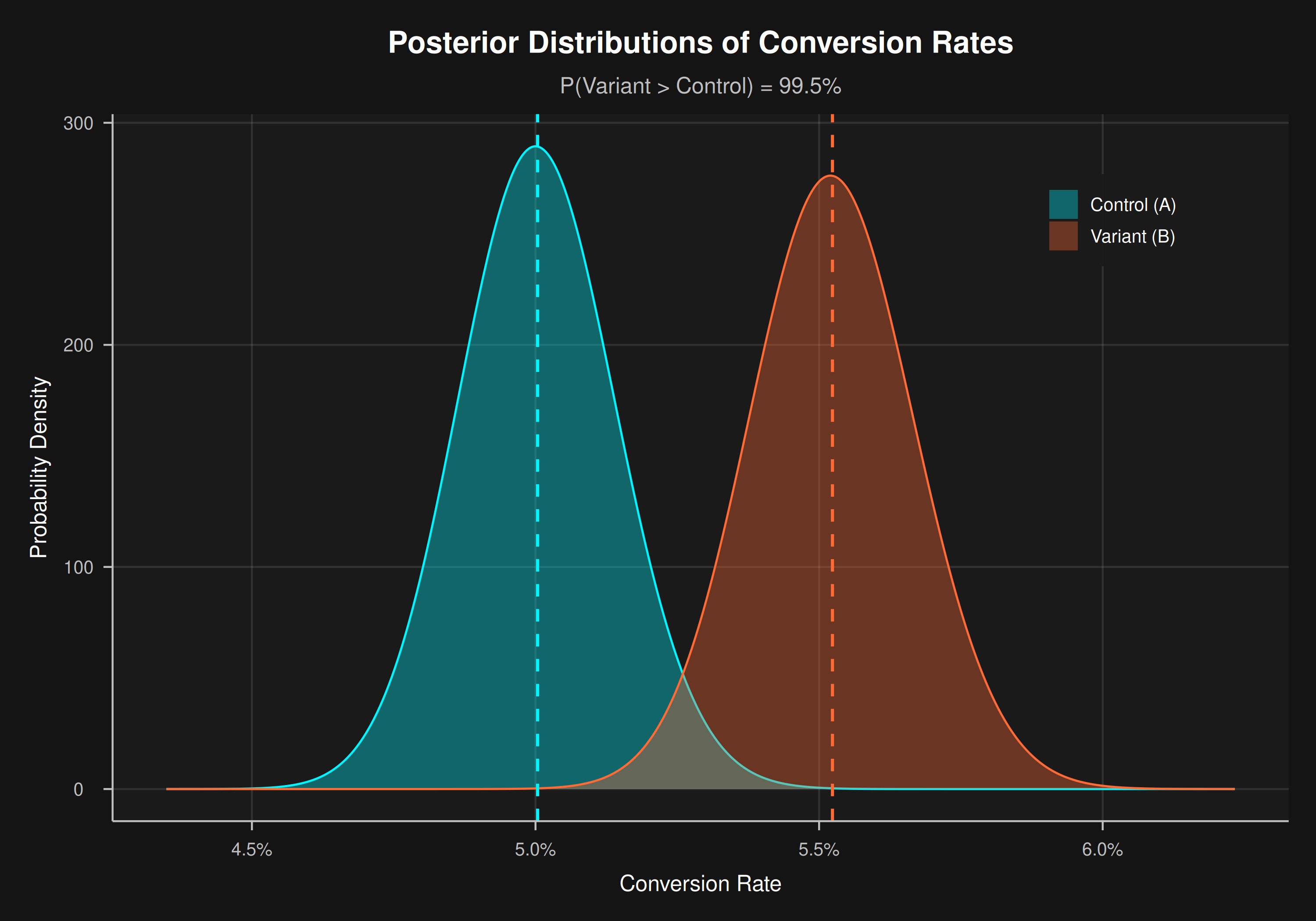
Posterior distributions showing Control (A) and Variant (B) conversion rates

Posterior distributions for Control A (cyan) and Variant B (coral). The minimal overlap and dashed lines at the posterior means show clear separation between the two variants.

Quantifying the Relative Uplift

Beyond $P(\theta_B > \theta_A \mid D)$ , we want the full posterior distribution of the relative uplift:

$\delta = \frac{\theta_B - \theta_A}{\theta_A}$

This gives us the expected percentage improvement and allows us to answer questions like "what's the probability the uplift exceeds 5%?"

# Calculate relative uplift distribution
uplift_samples = (variant_samples - control_samples) / control_samples

# Summary statistics
print(f"Expected uplift: {uplift_samples.mean():.1%}")
print(f"95% credible interval: [{np.percentile(uplift_samples, 2.5):.1%}, {np.percentile(uplift_samples, 97.5):.1%}]")
print(f"P(uplift > 5%): {(uplift_samples > 0.05).mean():.1%}")

# Output:
# Expected uplift: 10.5%
# 95% credible interval: [2.5%, 19.0%]
# P(uplift > 5%): 90.7%

This tells us:

We expect about a 10.5% relative improvement
There's a 95% probability the true uplift is between 2.5% and 19.0%
There's a 90.7% probability the uplift exceeds our 5% threshold of practical importance

Expected Loss: Decision Theory

The most powerful Bayesian concept for decision-making is expected loss. If we choose variant B, we incur a loss when $\theta_A > \theta_B$ . The expected loss is:

$\mathcal{L}(\text{choose B}) = \mathbb{E}[\max(\theta_A - \theta_B, 0) \mid D]$

This integral over the posterior is estimated via Monte Carlo:

$\mathcal{L}(\text{choose B}) \approx \frac{1}{N} \sum_{i=1}^{N} \max(\theta_A^{(i)} - \theta_B^{(i)}, 0)$

Expected loss has a natural interpretation: it's the average conversion rate we sacrifice by choosing the wrong variant, weighted by the probability of being wrong.

def expected_loss(winner_samples, loser_samples):
    """Calculate expected loss if we choose the 'winner'."""
    loss_if_wrong = np.maximum(loser_samples - winner_samples, 0)
    return loss_if_wrong.mean()

loss_choosing_b = expected_loss(variant_samples, control_samples)
loss_choosing_a = expected_loss(control_samples, variant_samples)

print(f"Expected loss if we ship B: {loss_choosing_b:.4%}")
print(f"Expected loss if we ship A: {loss_choosing_a:.4%}")

# Output:
# Expected loss if we ship B: 0.0003%
# Expected loss if we ship A: 0.5204%

The expected loss of shipping B is 0.0003% vs 0.52% for sticking with A. The decision is clear.

Stopping Rules

Bayesian methods offer more flexibility in monitoring experiments, though care is still needed. Common stopping criteria:

Probability threshold: Stop when $P(\theta_B > \theta_A \mid D) > 0.95$ or $< 0.05$
Expected loss threshold: Stop when $\min(\mathcal{L}(\text{choose A}), \mathcal{L}(\text{choose B})) < \varepsilon$ (e.g., $\varepsilon = 0.001$ )
Precision threshold: Stop when the 95% credible interval width for $\delta$ falls below a threshold

The expected loss criterion is particularly useful as it directly bounds the cost of a wrong decision.

def should_stop_test(variant_samples, control_samples,
                     prob_threshold=0.95, loss_threshold=0.001):
    """Determine if we have enough evidence to stop."""
    prob_b_better = (variant_samples > control_samples).mean()
    exp_loss_b = expected_loss(variant_samples, control_samples)
    exp_loss_a = expected_loss(control_samples, variant_samples)

    # Stop if clear winner with low expected loss
    if prob_b_better > prob_threshold and exp_loss_b < loss_threshold:
        return True, 'B', prob_b_better, exp_loss_b
    if prob_b_better < (1 - prob_threshold) and exp_loss_a < loss_threshold:
        return True, 'A', 1 - prob_b_better, exp_loss_a

    return False, None, prob_b_better, min(exp_loss_a, exp_loss_b)

Conclusion

Bayesian A/B testing provides:

Intuitive probability statements that stakeholders understand
Continuous monitoring without statistical penalties
Expected loss for risk-aware decision making
Full uncertainty quantification via posterior distributions

The key insight: instead of asking "is there a statistically significant difference?", we ask "what's the probability B is better, and by how much?"

For most business decisions, that's exactly what you need to know.

We Can Help

Need help implementing Bayesian testing in your organisation? KH Solve can build the infrastructure, run the analysis, and help you make better decisions. Get in touch.