Storm Desmond: A Once in Century Storm?

Modelling Extreme River Flows with Bayesian Statistics

During my PhD, I worked heavily with Extreme Value Theory (EVT) and always found it fascinating. The extremes in data are a crucial part of the data and can give us important insights that can guide decision making. EVT can tell us the probability of a 1-in-100 year flood that overwhelms defences or a peak demand that crashes servers. These rare events carry consequences far exceeding their frequency and understanding them can be the difference between being prepared and being caught out.

In this post, I'll walk through a complete EVT analysis of UK river flow data, demonstrating how Bayesian methods help us quantify our uncertainty around rare events.

The Data: River Tyne at Bywell

We're analysing river flow records from the River Tyne at Bywell, near Newcastle Upon Tyne with hydrological records spanning 68 years (1956-2024). The data comes from the National River Flow Archive (NRFA), which provides both annual maxima (AMAX) and peaks-over-threshold (POT) series.

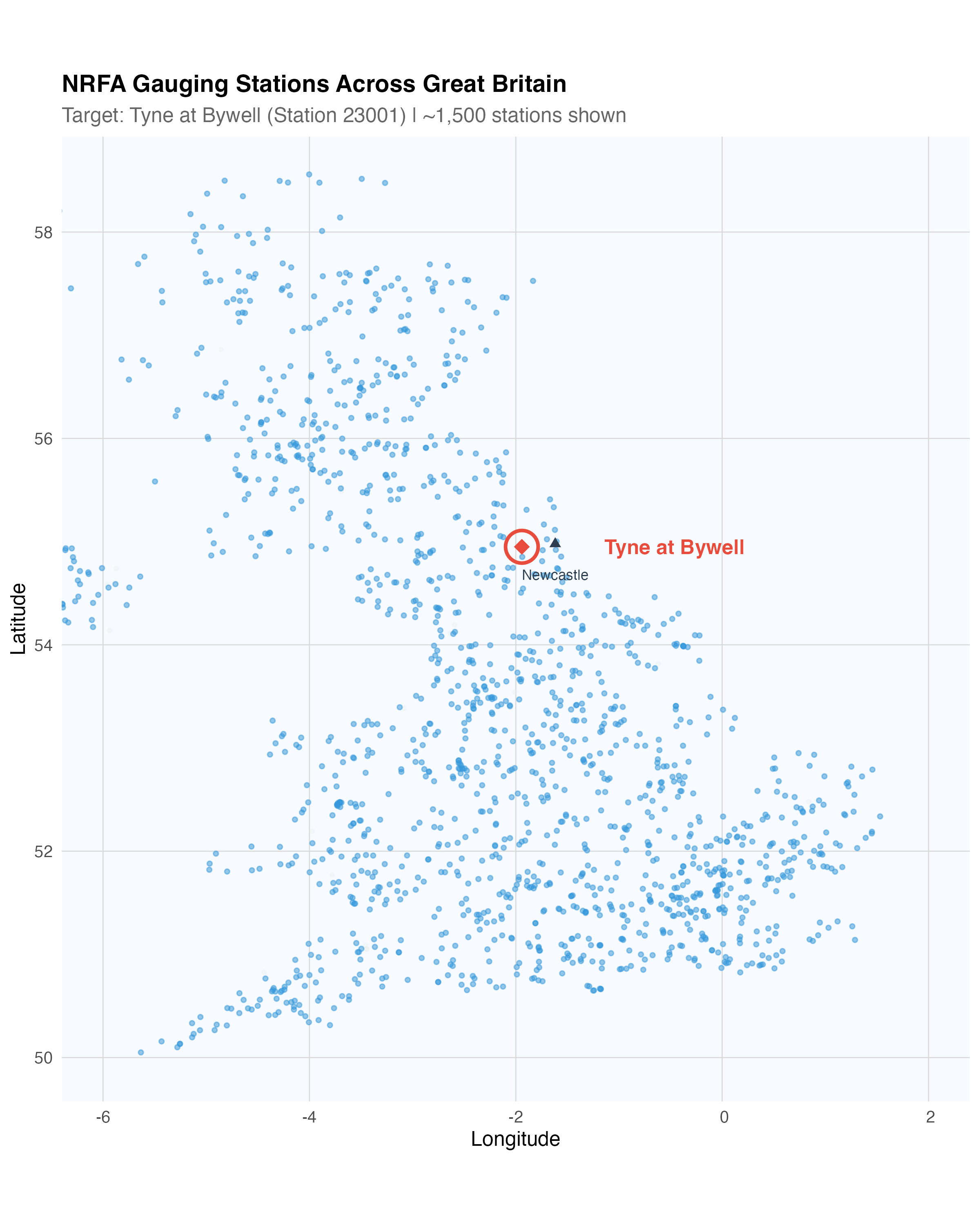
Map showing NRFA gauging stations across Great Britain, with Tyne at Bywell highlighted.

The record includes some notable events, most dramatically Storm Desmond in December 2015, which produced a peak flow of 1,729 m³/s - the highest in the 68-year record.

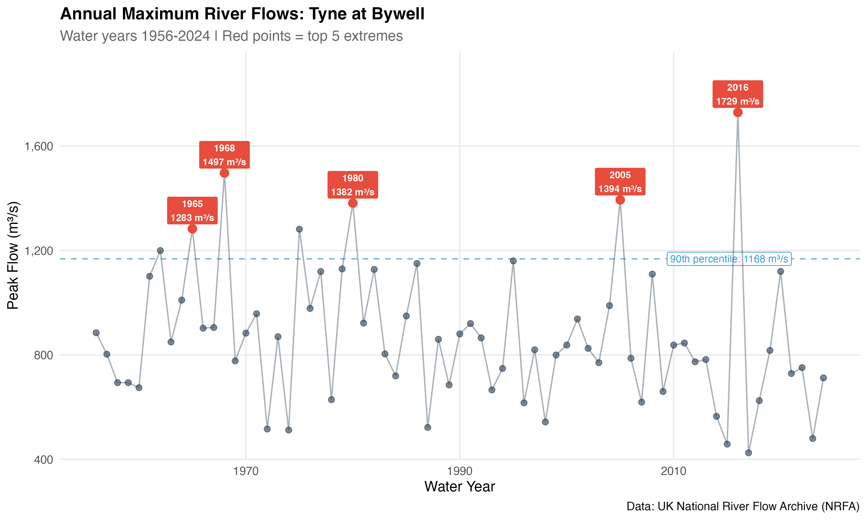
Annual maximum flows showing the top 5 extremes, including Storm Desmond.

Note: UK hydrological data uses water year (1 Oct - 30 Sep) to align with flood season. Storm Desmond (Dec 2015) falls in water year 2016.

The GEV Distribution: Modelling Block Maxima

The Generalised Extreme Value (GEV) distribution is the theoretically justified model for block maxima. It has three parameters:

• Location ($\mu$): The "typical" annual maximum (~785 m³/s)
• Scale ($\sigma$): The spread of annual maxima (~201 m³/s)
• Shape ($\xi$): Determines tail behaviour - the crucial parameter

The shape parameter tells us whether extreme flows have a hard upper limit ($\xi < 0$), follow an exponential-type tail ($\xi = 0$), or have a heavy, unbounded tail ($\xi > 0$).

For the Tyne, our Bayesian estimate gives $\xi = -0.020$ with a 95% credible interval of $(-0.17, +0.18)$. This spans zero, therefore we can't confidently distinguish between bounded and unbounded tail behaviour with 68 years of data.

This uncertainty matters, and it's precisely why we use Bayesian methods.

Why Bayesian?

Traditional (frequentist) approaches give you a point estimate and a confidence interval. But there's a subtlety: a 95% confidence interval doesn't mean "95% probability the true value lies here." It's a statement about the procedure, not the parameter.

Bayesian methods give you something more useful - a full posterior distribution representing our uncertainty about the parameter given the data we observed. This matters for EVT in several ways:

1. Direct probability statements: A Bayesian 95% credible interval actually means "95% probability the parameter lies in this range." Much more intuitive for decision-making.
2. Small sample honesty: With only 68 annual maxima, asymptotic approximations can be unreliable. MCMC-based Bayesian inference doesn't depend on large-sample theory.
3. Full uncertainty propagation: The posterior uncertainty in parameters flows naturally into uncertainty in return levels. The return levels give the full distribution of plausible 100-year flows.
4. Any percentile you need: Want the 90th percentile of the 100-year return level for conservative planning? The posterior gives you that directly.
5. Shape parameter stability: The GEV shape parameter is difficult to estimate with MLE, especially for small samples. Bayesian estimation with sensible priors is more stable.

When you're trying to make decisions about rare events with limited data, Bayesian methods give you every tool that helps you honestly represent what you know and don't know.

Return Levels: What's the 100-Year Flow?

The question everyone wants answered: how big is a 1-in-100 year flow?

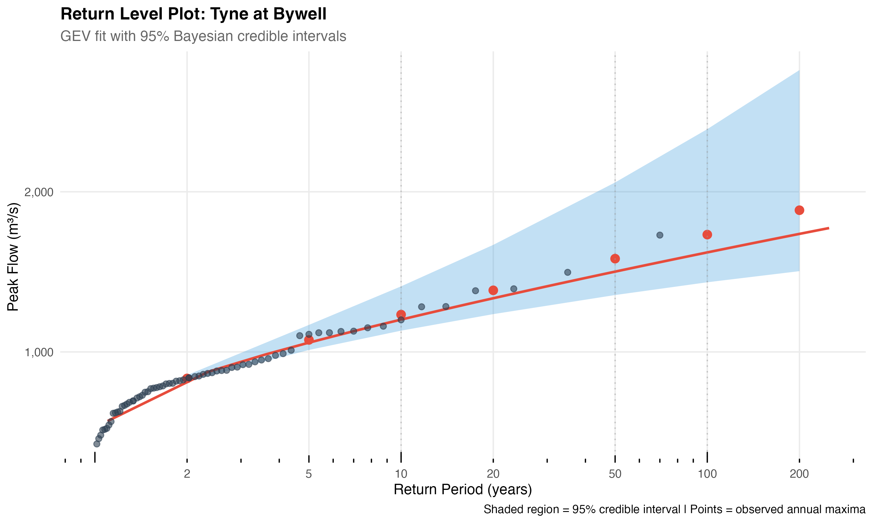
Return level plot showing GEV fit with 95% Bayesian credible intervals. The shaded region captures our uncertainty.

Understanding the Return Level Plot:

• The grey points are observed annual maxima - one per year from our 69-year record. Their horizontal position shows empirical return period (how often we'd expect a flow that size based purely on the historical ranking). Storm Desmond sits at the top right.
• The red curve is the fitted GEV distribution (maximum likelihood estimate), showing expected flow magnitude at any return period. It curves upward because larger flows become increasingly rare.
• The red points with uncertainty bands are the Bayesian estimates at key return periods (10, 50, 100 years etc.). These differ slightly from the MLE curve because they account for parameter uncertainty - particularly in the shape parameter, which strongly influences extrapolation.
• Why show MLE curve but Bayesian points? The MLE curve is a single "best fit" line. The Bayesian approach produces a full distribution of plausible curves (one for each posterior sample), not a single line. Hence, we summarise this by showing the posterior mean and credible intervals at specific return periods.

Our estimates (posterior means with 95% credible intervals):

Return Period	Estimated Flow	95% Credible Interval
10-year	1,224 m³/s	1,122 - 1,377
50-year	1,573 m³/s	1,354 - 2,002
100-year	1,723 m³/s	1,436 - 2,338

Notice how uncertainty grows with return period. For the 100-year flow, we're 95% confident it lies somewhere between 1,436 and 2,338 m³/s - a range of nearly 1,000 m³/s. This isn't a failure of the analysis; it's an honest reflection of what 68 years of data can tell us about events we expect once per century.

Storm Desmond in context: At 1,729 m³/s, Storm Desmond sits almost exactly at our 100-year estimate. The models suggest it was roughly a 1-in-100 year event - rare, but not unprecedented.

The GPD Alternative: Peaks Over Threshold

Annual maxima give us just 68 data points. But flow events exceeding a high threshold occur more frequently, such that the NRFA provides 301 such events over the same period.

The Generalised Pareto Distribution (GPD) models these threshold exceedances. Mathematically, GEV and GPD are linked - if annual maxima follow a GEV, then threshold exceedances follow a GPD with the same shape parameter.

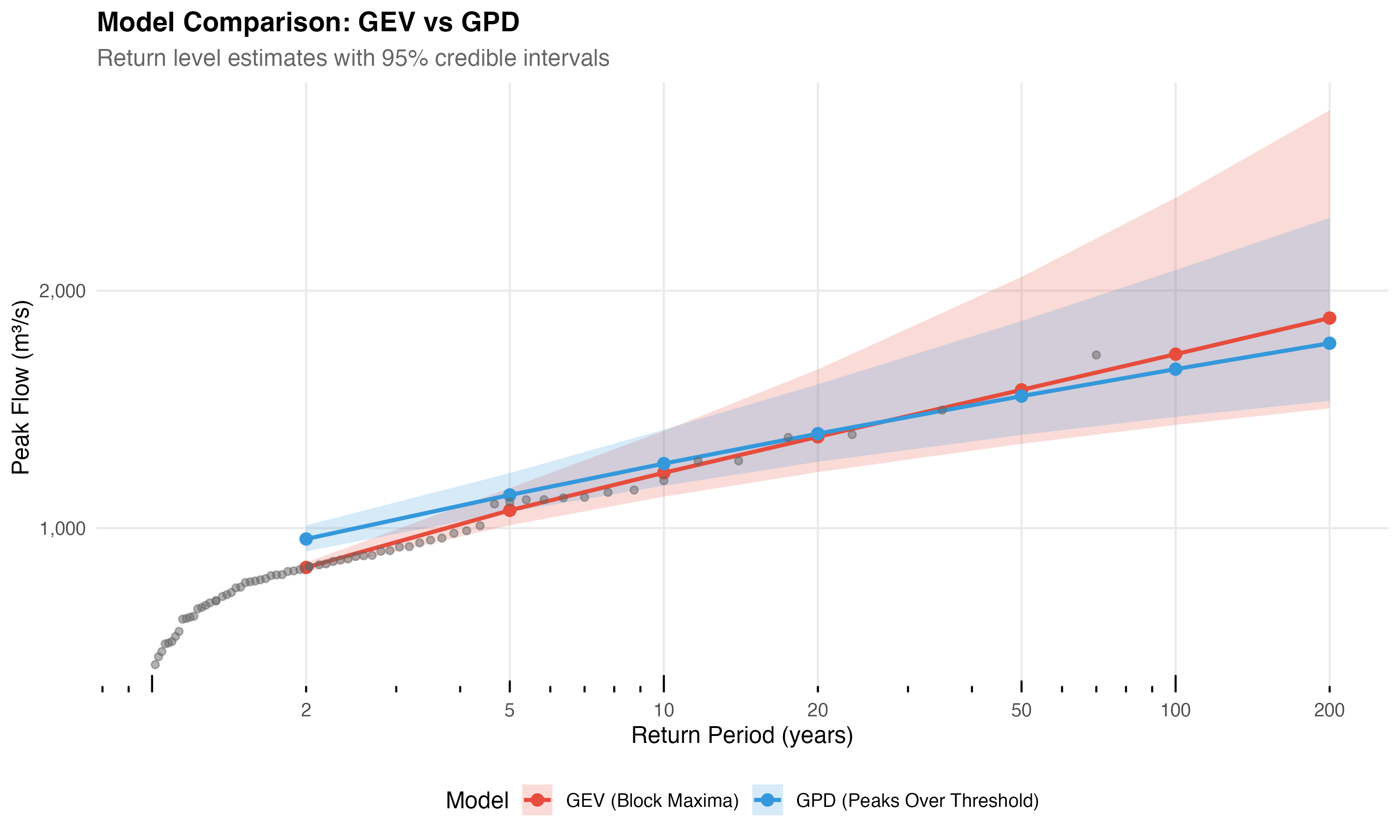
Comparison of GEV and GPD return level estimates. The models agree within 5% for most return periods.

Return Period	GEV (m³/s)	GPD (m³/s)	Difference
10-year	1,224	1,270	+4%
50-year	1,573	1,554	-1%
100-year	1,723	1,668	-3%

The agreement is reassuring - two different approaches, using different subsets of the data, give consistent answers. Both suggest the 100-year flow is around 1,700 m³/s.

Planning with Uncertainty

Here's where Bayesian analysis becomes genuinely useful for decision-making. The posterior distribution doesn't just give us a best estimate, it gives us the full range of plausible values.

We're modelling peak river flows which ultimately determine whether defences are overtopped. Consider planning flow defences for a 100-year return level. Which value do you use?

Posterior Percentile	100-year Estimate	Planning Implication
50th (median)	1,688 m³/s	"Best guess" - 50% chance of underestimating
75th	1,888 m³/s	More conservative - 25% chance of underestimating
95th	2,338 m³/s	Highly conservative - 5% chance of underestimating

A residential flood wall might use the median estimate. Critical infrastructure, a hospital or a power station, might demand the 95th or even the 99th percentile. The statistics inform the decision; they don't make it.

Where Else Does EVT Apply?

The same framework applies wherever rare events drive risk:

Established Applications

• Financial risk (Value at Risk, extreme losses)
• Insurance pricing for catastrophic claims
• Engineering reliability (component failure under extreme loads)

Emerging Applications

• Cybersecurity: sizing defences for the "100-year" DDoS attack
• Supply chain: planning inventory for extreme demand spikes
• Cloud infrastructure: capacity planning for viral traffic surges
• Healthcare: hospital surge capacity for pandemic events

The Peaks Over Threshold approach is particularly relevant for business data, for example, fraud alerts, system alerts, insurance claims above a deductible.

Key Takeaways

1. Extremes can be hugely informative - definitely worth modelling (for insights and fun)
2. Uncertainty grows with rarity - a 100-year estimate has wide confidence intervals, and that's honest, not a limitation
3. Bayesian methods help quantify what we don't know - the full posterior distribution supports risk-informed decision making
4. GEV and GPD provide complementary views - agreement between them increases confidence in results
5. The framework generalises - any domain with rare, high-consequence events can benefit from EVT

We Can Help

Need help applying Extreme Value Theory to your domain? KH Solve can run the analysis, quantify your tail risks, and help you make better decisions under uncertainty. Get in touch.

---

References

1. National River Flow Archive. Tyne at Bywell (Station 23001). UK Centre for Ecology & Hydrology. Data